


Charting Change: Using an XmR Chart
Mark Graban’s blog post, “What Do We Learn from Charting a Reduction in CLABSI Rates in Different Ways?”, provides a great example of how to plot and analyze data.
Here I present my analysis, observations, and comments.
The data, which appears to be a count of central line associated blood stream infections (CLABSI) for each year starting 2005 and on through 2017, is shown in Table 1. According to Mark, it was presented by some leaders from a children’s hospital.
Table 1. Data for neonatal intensive care unit (NICU) central line associated blood stream infections (CLABSI) for 2005-2017

The simplest analysis that provides insight is the best analysis to perform. So, let’s plot the data (Figure 1).
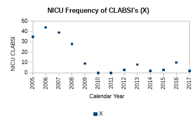 Figure 1. Plot of count of central line associated blood stream infections (CLABSI) for 2005-2017
It is obvious just from the plot in Figure 1 that the performance of the system has changed; it has improved. It has dropped from ~40 NICU CLABSIs for 2005-2007 to ~6 NICU CLABSIs for 2009-2017. Mark writes that a process change was made around 2008. However, no other details are available as to the nature of the change. Without further context all we can say is that the effect of the change made in 2008 in subsequent years is obvious and dramatic—evidence of effectiveness of action. No calculations were necessary to make this observation.
Still, we could add a center line to the plot (Figure 2) to gain further insight.
 Figure 2. The addition of the center line (average of all 13 points), clearly shows two distinct runs: a run of four points for 2005-2008, and a run of nine points for 2009-2017. The run of nine points is unusual, and signals a process shift.
The center line is the mean, calculated using all 13 points. It is ~14. From the plot we see a run of four points above the mean and a run of nine points below the mean. The second run is unusual and signals a process shift. It supports the claim that a process change was made around 2008-2009. With a single calculation, the mean, we have corroborated our original observation.
If we want to predict the performance of the system in 2018 or 2019 or 2020, we need to construct an XmR chart. Knowing that there was a process change around 2008, we should focus on the system’s performance after that i.e. 2009 and beyond. Table 2 shows the calculations for the XmR chart.
Table 2. Calculations are shown for attributes necessary to plot an XmR chart. The calculations are shown just for the process thought to currently exist i.e. 2009-2017

The moving range (mR) is calculated as the absolute value of the difference between the current and previous year e.g. mR for 2010 is calculated as |X2010 – X2009| = |0 – 9|, which is 9.
The mean value is calculate for just those points after the process change, i.e. 2009-2017, as (9+0+0+3+8+2+3+10+2)/9 = 37/9 = 4.1
The mean moving range is calculate as the average of all the calculated moving range values as (9+0+3+5+6+1+7+8)/8 = 39/8 = 4.9
The upper natural limit (UNL) is calculated as the mean + 2.66*mean range i.e. 4.1 + 2.66*4.9 = 17
The lower natural limit (LNL) is calculate as the mean – 2.66*mean range i.e. 4.1 – 2.66*4.9 = -9. However, because you cannot have negative count, the LNL is set to zero on the chart.
The upper range limit (URL) is calculated as 3.268*mean range i.e. 3.268*4.9 = 15.9
The lower range limit (LRL) is zero.
The XmR chart is shown in Figure 3.
 Figure 3. The natural process limits are shown for the current system with the UNL = 17, mean = 4.1, and LNL = 0. If the system continued to perform without change, we can expect between 0 and 17 CLABSIs in the next years.
From the XmR chart we can make the following predictions:
Provided the system continues to operate as it has the past few years, we can expect an average of ~4 CLABSIs in future years. There may be years where we could see up to ~17 CLABSIs. There may be years where there are none. Further more we can expect the counts to vary by ~5 on average from one year to the next. Some years may vary by as much as 16 counts. Others may not vary at all.
Management must decide whether this is adequate performance. If further reduction in NICU CLABSIs is wanted, new actions to improve the current system will need to be taken.
Links
[1] Graban, Mark. What Do We Learn from Charting a Reduction in CLABSI Rates in Different Ways?. Retrieved on 2017.11.01 from https://www.leanblog.org/2017/11/learn-charting-reduction-clabsi-rates-different-ways/
Understanding How You Fit In

Early on in my career my thoughts about the world and work were fragmentary. They often conflicted with one another. These conflicting disorganized thoughts were the source of a lot of confusion and frustration.
Then I read W. Edwards Deming’s Out of the Crisis[1]. On page 4, Fig. 1 shows a diagram of “Production viewed as a system”. It instantly reshaped my perspective. I had an “Aha!” moment. It gave me the context to understand my differentiated knowledge and experience. I understood where and how I fit in.
I sense that most people suffer from confusion and frustration from a lack of context for what they do. While I believe everyone should buy and read Out of the Crisis, it is not an easy read for the new worker.
This year I discovered two books that I feel are more accessible: Improving Performance Through Statistical Thinking[2] and Statistical Thinking: Improving Business Performance[3]. Both provide the worker a frame for understanding their job, how it fits within an organization, and how to work better, both individually and together.
These books aren’t just for quality people. In fact I think they are more helpful to everyone else–Marketing, R&D, Design & Development, Manufacturing, Sales, Accounting, Finance, Legal, and any other department I might have missed. I think every worker who reads them will have an “Aha!” moment, and can immediately benefit from them.
Dr. Deming pointed out, “It is not enough to do your best; you must know what to do, and then do your best.” You already do your best, but with confusing and frustrating results. These books are wonderful resources to help you understand what you should do so that your best efforts produce satisfying results; ones that make you feel good and proud.
I feel it’s important for me to say this: Don’t let the reference to Statistics in their titles scare you off. You don’t need to know any Statistics to read them. In fact, I feel you will benefit more if you didn’t know any Statistics. You will learn three important lessons from these books:
- All work occurs in a system of interconnected processes
- Variation exists in all processes, and
- Understanding and reducing variation are keys to success
Links
[1] Deming, W. Edwards. Out of the Crisis. Cambridge, MA: Center for Advanced Engineering Study, MIT. 1991. Print. ISBN 0-911379-01-0
[2] Britz, Galen C., Donald W. Emerling, Lynne B. Hare, Roger W. Hoerl, Stuart J. Janis, and Janice E. Shade. Improving Performance Through Statistical Thinking. Milwaukee, WI: ASQ Quality Press. 2000. Print. ISBN 0-87389-467-7
[3] Hoerl, Roger, and Ronald D. Snee. Statistical Thinking: Improving Business Performance. Pacific Grove, CA: Duxbury, Thomson Learning. 2002. Print. ISBN 0-534-38158-8
On Variation and Some of its Sources

Virtually every component is made to be assembled with its counterpart(s) into sub-assemblies and final assemblies.
If individual pieces of a given component could be made identical to one another, then they would either all conform or all fail to conform to the component’s design requirements. If they conform, then we could pick a piece at random for use in a sub- or final-assembly. It would fit and function without fail, as intended.
But material varies, machine operation varies, the work method varies, workers vary, measurement varies, as does the environment. Such variation, especially in combination, makes it impossible to produce anything identical. Variation is a fundamental principle of nature. All things vary.
Variation affects the fit, the form and the function of a component. And, it is propagated along the assembly line such that the final product is at times a mixed bag of conforming and nonconforming widgets.
Material Consider 316 Stainless Steel. It is used to make medical devices. Manufacturers buy it from metal producers in sheet stock or bar stock.
If we measured the dimensional attributes of the received stock, e.g. its diameter or length, for several different purchase orders, we would see that they were not identical between orders. They vary. If we measured these attributes for pieces received in a single order, we would see that they were not identical between pieces of that order either. If we measured these attributes for a single piece at different points in its cross-section, we would see that they, too, were not identical. If we then zoomed in to investigate the crystalline structure of the stainless steel, we would see that the crystals were not identical in shape or size.
The elemental composition, in percent by weight, of 316 Stainless Steel is: 0.08% Carbon, 2.00% Manganese, 0.75% Silicon, 16.00-18.00% Chromium, 10.00-14.00% Nickel, 2.00-3.00% Molybdenum, 0.045% Phosphorous, 0.030% Sulfur, 0.10% Nitrogen, and the balance is Iron. We see that the amount of Chromium, Nickel, Molybdenum and Iron are specified as ranges i.e. they are expected to vary within them by design!
These are some of the ways a specific raw material used in the production of medical devices varies. Keep in mind that a medical device isn’t a single component but an assembly of several components likely made of different materials that will vary in just such ways as well. All this variation affects the processing (i.e. machining, cleaning, passivation, etc.) of the material during manufacturing, as well as the device performance in use.
Machine One piece of equipment used in the production of medical device components is the CNC (Computer Numerical Control) machine. Its condition, as with all production equipment, varies with use.
Take the quality of the lubricating fluid: it changes properties (e.g. its viscosity) with temperature thus affecting its effectiveness. The sharpness of the cutting tool deteriorates with use. A component made with a brand new cutting tool will not be identical to one made from a used cutting tool whose cutting edges have dulled. The cutting is also affected by both the feed-rate and the rotation-rate of the cutting tool. Neither of which remain perfectly constant at a particular setting.
What’s more, no two machines perform in identical ways even when they are the same make and model made by the same manufacturer. In use, they will almost never be in the same state as each other, with one being used more or less than the other, and consumables like cutting tools in different states of wear. Such variability will contribute to the variability between the individual pieces of the component.
Method Unless there is standardized work, we would all do the work in the best way we know how. Each worker will have a best way slightly different from another. Variation in best ways will find its way into the pieces made using them.
These days a production tool like a CNC machine offers customized operation. The user can specify the settings for a large number of operating parameters. Users write “code” or develop a “recipe” that specifies the settings for various operating parameters in order to make a particular component. If several such pieces of code or recipes exist, one different from another, and they are used to make a particular component, they will produce pieces of that component that vary from one to another.
When and how an adjustment is made to control parameters of a tool will affect the degree of variation between one piece and another. Consider the method where a worker makes adjustment(s) after each piece is made to account for its deviation from the target versus one where a worker makes an adjustment only when a process shift is detected. Dr. Deming and Dr. Wheeler have shown that tampering with a stable process, as the first worker does, will serve to increase the variation in the process.
All such variation in method will introduce variability into the manufactured pieces.
Man There are a great many ways in which humans vary physically from one another. Some workers are men, others are women. Some are short, others are tall. Some are young, others are older. Some have short fat fingers, others have long thin fingers. Some have great eyesight, others need vision correction. Some have great hearing, others need hearing aids. Some are right handed, others are left handed. Some are strong, others not so much. Some have great hand-eye coordination, others do not. We all come from diverse ethnic backgrounds.
Not all workers have identical knowledge. Some have multiple degrees, others are high school graduates. Some have long experience doing a job, others are fresh out of school. Some have strong knowledge in a particular subject, others do not. Some have deep experience in a single task, others have shallow experience. Some have broad experience, others have focused experience.
Last, but not least, we all bring varying mindsets to work. Some may be intrinsically motivated, others need to be motivated externally. Some may be optimists, others may be pessimists. Some want to get better everyday, others are happy where they are. Some like change, others resist it. Some are data driven, others use their instinct.
All this variation affects the way a job gets done. The variation is propagated into the work and ultimately manifests itself in the variation of the manufactured component.
Measurement We consider a measured value as fact, immutable. But that’s not true. Measuring the same attribute repeatedly does not produce identical results between measurements.
Just like production tools, measurement tools wear from use. This affects the measurement made with it over the course of its use.
And also just like production tools, the method (e.g. how a part is oriented, where on the part the measurement is made, etc.) used to make a measurement affects the measured value. There is no true value of any measured attribute. Different measurement methods produce different measurements of the same attribute.
So even if by chance two pieces were made identical we wouldn’t be able to tell because of the variability inherent in the measurement process.
Environment Certain environmental factors affect all operations regardless of industry. One of them is time. It is not identical from one period to the next. Months in a year are not identical in duration. Seasons in a year are different from one another. Daytime and nighttime are not identical to one another. Weekdays and weekends are not identical to one another.
Even in a climate controlled facility the temperature cycles periodically around a target. It varies between locations as well. Lighting changes over the course of the day. Certain parts of the workplace may be darker than others. Noise, too, changes over the course of the day: quiet early in the morning or into the night, and noisier later into the day. There is variation in the type of noise, as well. Vibration by definition is variation. It can come from a heavy truck rolling down the street or the motor spinning the cutting tool in a production machine. Air movement or circulation isn’t the same under a vent as compared to a spot away from a vent, or when the system is on versus when it is off.

The 5M+E (Material, Machine, Method, Man, Measurement, and Environment) is just one way to categorize sources of variation. The examples in each are just a few of the different sources of variation that can affect the quality of individual pieces of a component. While we cannot eliminate variation, it is possible to systematically reduce it and achieve greater and greater uniformity in the output of a process. The objective of a business is to match the Voice of the Customer (VOC) and the Voice of the Process (VOP). The modern day world-class definition of quality is run-to-target with minimal variation!
“Our approach has been to investigate one by one the causes of various “unnecessaries” in manufacturing operations…”
— Taiichi Ohno describing the development of the Toyota Production System
Links
[1] Kume, Hitoshi. Statistical Methods for Quality Improvement. Tokyo, Japan: The Association for Overseas Technical Scholarship. 2000. Print. ISBN 4-906224-34-2
[2] Monden, Yasuhiro. Toyota Production System. Norcross, GA: Industrial Engineering and Management Press. 1983. Print. ISBN 0-89806-034-6
[3] Wheeler, Donald J. and David S. Chambers. Understanding Statistical Process Control. Knoxville, TN: SPC Press, Inc. 1986. Print. ISBN 0-945320-01-9
Reliability, Confidence, and Sample Size, Part II

In Part I the problem was to find the sample size, n, given failure count, c = 0, confidence level = 1 – P(c = 0), and minimum reliability = (1 – p’). The table giving sample size, n, with failures c = 0, for certain common combinations of confidence level and minimum reliability is reproduced below.

While I would like that none of the samples fail testing, failures do happen. Does that mean testing should stop on first fail? Are the test results useless? In this part I will flip the script. I will talk about what value I can extract from test results if I encounter one or more failures in the test sample.
I start with the binomial formula as before

It gives us the likelihood, P(x = c), of finding exactly c failures in n samples for a particular population failure rate p’. (Note that 1 – P(x ≤ c) is our confidence level, and 1 – p’ = q’ is our desired reliability.)
However, knowing the likelihood of finding just c failures in n samples isn’t enough. Different samples of size n from the same population will give different counts of failures c. If I am okay with c failures in n samples, then I must be okay with less than c failures, too! Therefore, I need to know the cumulative likelihood of finding c or less failures in n samples, or P(x ≤ c). That likelihood is calculated as the sum of the individual probabilities. For example, if c = 2 samples fail, I calculate P(x ≤ 2) = P(x = 2) + P(x = 1) + P(x = 0).
For a particular failure rate p’, I can make the statement that my confidence is 1 – P(x ≤ c) that the failure rate is no greater than p’ or alternatively my reliability is no less than q’ = (1 – p’).
It is useful to build a plot of P(x ≤ c) versus p’ to understand the relationship between the two for a given sample size n and failure count c. This plot is referred to as the operating characteristic (OC) curve for a particular n and c combination.
For example, given n = 45, and c = 2, my calculations would look like:


The table below shows a few values that were calculated:

A plot of P(c ≤ 2) versus p’ looks like:

From the plot I can see that the more confidence I require, the higher the failure rate or lesser the reliability estimate will be (e.g. 90% confidence with 0.887 reliability, or 95% confidence with 0.868 reliability.) Viewed differently, the more reliability I require, the less confidence I have in my estimate (e.g. 0.95 reliability with 40% confidence level).
Which combination of confidence and reliability to use depends on the user’s needs. There is no prescription for choosing one over another.
I may have chosen a sample size of n = 45 expecting c = 0 failures for testing with the expectation of having 90% confidence at 0.95 reliability in my results. But just because I got c = 2 failures doesn’t mean the effort is for naught. I could plot the OC curve for the combination of n, and c to understand how my confidence and reliability has been affected. Maybe there is a combination that is acceptable. Of course, I would need to explain why the new confidence, and reliability levels are acceptable if I started with something else.
Operating characteristic curves can be constructed in MS Excel or Libre Calc with the help of BINOM.DIST(c, n, p’, 1) function.

Once I have values for p’ and P(c ≤ 2), I can create an X-Y graph with X = p’, and Y = P(c ≤ 2).
Links
[1] Burr, Irving W. Elementary Statistical Quality Control. New York, NY: Marcel Dekker, Inc. 1979. Print. ISBN 0-8247-6686-5
Reliability, Confidence, and Sample Size, Part I
 Say I have designed a widget that is supposed to survive N cycles of stress S applied at frequency f.
I can demonstrate that the widgets will conform to the performance requirement by manufacturing a set of them and testing them. Such testing, though, runs headlong into the question of sample size. How many widgets should I test?
For starters, however many widgets I choose to test, I would want all of them to survive i.e. the number of failures, c, in my sample, n, should be zero. (The reason for this has more to do with the psychology of perception than statistics.)
If I get zero failures (c = 0) in 30 samples (n = 30), does that mean I have perfect quality relative to my requirement? No, because the sample failure rate, p = 0/30 or 0%, is a point estimate for the population failure rate, p’. If I took a different sample of 30 widgets from the same population, I may get one, two, or more failures.
The sample failure rate, p, is the probability of failure for a single widget as calculated from test data. It is a statistic. It estimates the population parameter, p’, which is the theoretical probability of failure for a single widget. The probability of failure for a single widget tells us how likely it is to fail the specified test.
If we know the likelihood of a widget failing the test, p’, then we also know the likelihood of it surviving the test, q’ = (1 – p’). The value, q’, is also known as the reliability of the widget. It is the probability that a widget will perform its intended function under stated conditions for the specified interval.
The likelihood of finding c failures in n samples from a stable process with p’ failure rate is given by the binomial formula.

But here I am interested in just the case where I find zero failures in n samples. What is the likelihood of me finding zero failures in n samples for a production process with p’ failure rate?


If I know the likelihood of finding zero failure in n samples from a production process with p’ failure rate, then I know the likelihood of finding 1 or more failures in n samples from the production process, too. It is P(c ≥ 1) = 1 – P(0). This is the confidence with which I can say that the failure rate of the production process is no worse than p’.
Usually a lower limit is specified for the reliability of the widget. For example, I might want the widget to survive the test at least 95% of the time or q’ = 0.95. This is the same as saying I want the failure rate to be no more than p’ = 0.05.
I would also want to have high confidence in this minimum reliability (or maximum failure rate). For example, I might require 90% confidence that the minimum reliability of the widget is q’ = 0.95.
A 90% confidence that the reliability is at least 95% is the same as saying 9 out of 10 times I will find one or more failures, c, in my sample, n, if the reliability were less than or equal to 95%. This is also the same as saying that 1 out of 10 times I will find zero failures, c, in my sample, n, if the reliability were less than or equal to 95%. This, in turn, is the same as saying P(0) = 10% or 0.1 for p’ = 0.05.
With P(0) and p’ defined, I can calculate the sample size, n, that will satisfy these requirements.


The formula can be used to calculate the sample size for specific values of minimum reliability and confidence level. However, there are standard minimum reliability and confidence level values used in industry. The table below provides the sample sizes with no failures for some standard values of minimum reliability and confidence level.
What should the reliability of the widget be? That depends on how critical its function is.
What confidence level should you choose? That again depends on how sure you need to be about the reliability of the widget.
Note: A basic assumption of this method is that the failure rate, p’, is constant for all the widgets being tested. This is only possible if the production process producing these widgets is in control. If this cannot be demonstrated, then this method will not help you establish the minimum reliability for your widget with any degree of confidence.
Links
[1] Burr, Irving W. Elementary Statistical Quality Control. New York, NY: Marcel Dekker, Inc. 1979. Print. ISBN 0-8247-6686-5
Whose Measurement is Right?
 Every company I’ve worked for inspects the product it receives from its suppliers to determine conformance to requirements. The process is variously referred to as incoming inspection or receiving inspection.
Sometimes the receiving inspection process identifies a lot of product that fails to conform to requirements. That lot is subsequently classified as nonconforming material and quarantined for further review. There are many reasons why a lot of product may be classified as nonconforming. Here I wish to focus just on reasons having to do with measurement.
Once a company discovers nonconforming parts, it usually contacts its supplier to share that information. It is not unusual, however, for the supplier to push back when their data for the lot of product shows it to be conforming. So, how can a given lot of product be both conforming and nonconforming? Who is right?
We need to recognize that measurement is a process. The measured value is an outcome of this process. It depends on the measurement tool used, the skill of the person making the measurement and the steps of the measurement operation. A difference in any of these factors will show up as a difference in the measured value.
It is rare that a measurement process is the same between a customer and its supplier. A customer may use different measurement tools than its supplier. For example, where the customer might have used a caliper or micrometer, the supplier may have used an optical comparator or CMM. Even if both the customer and the supplier use the same measurement tool, the workers using that tool are unlikely to have been trained in its use in the same way. Finally, the steps used to make the measurement, such as fixturing, lighting and handling the part, which often depend on the measurement tool used, will likely be different, too.
Thus, more often than not, a measurement process between a supplier and a customer will be different. Each measured value is correct in its context—the supplier’s measurement is correct in its context, as is the customer’s measurement in its context. But because the measurement process is different between the two contexts, the measured values cannot be compared directly with one another. So it is possible that the same lot of product may be conforming per the supplier’s measurements and nonconforming per the customer’s measurements.
But why are we measuring product twice: once by the supplier and again by the customer? Measurement is a costly non-value adding operation, and doing it twice is excess processing–wasteful. One reason I’ve been told is this is done to confirm the data provided by the supplier. But confirmation is possible only if the measurement process used by the customer matches the one used by the supplier.
Besides, if we are worried about the quality of supplier data, we should then focus efforts on deeply understanding their measurement process, monitoring its stability and capability, and working with the supplier to improve it if necessary. With that we should trust the measurement data the supplier provides and base our decisions on it, and eliminate the duplicate measurement step during receiving inspection.
Links
[1] Eliminate Waste in Incoming Inspection: 10 ideas of where to look for waste in your process http://www.qualitymag.com/articles/92832-eliminate-waste-in-incoming-inspection Retrieved 2017-06-29
QSR Required Procedures
I have identified 40 procedures required by 21 CFR 820: the Quality System Regulation
- § 820.22 for quality audits…
- § 820.25(b) for identifying training needs…
- § 820.30(a)(1) to control the design of the device in order to ensure that specified design requirements are met
- § 820.30(c) to ensure that the design requirements relating to a device are appropriate and address the intended use of the device, including the needs of the user and patient
- § 820.30(d) for defining and documenting design output in terms that allow an adequate evaluation of conformance to design input requirements
- § 820.30(e) to ensure that formal documented reviews of the design results are planned and conducted at appropriate stages of the device’s design development
- § 820.30(f) for verifying the device design
- § 820.30(g) for validating the device design
- § 820.30(h) to ensure that the device design is correctly translated into production specifications
- § 820.30(i) for the identification, documentation, validation or where appropriate verification, review, and approval of design changes before their implementation
- § 820.40 to control all documents that are required by this part
- § 820.50 to ensure that all purchased or otherwise received product and services conform to specified requirements
- § 820.60 for identifying product during all stages of receipt, production, distribution, and installation to prevent mixups
- § 820.65 for identifying with a control number each unit, lot, or batch of finished devices and where appropriate components
- § 820.70(a) that describe any process controls necessary to ensure conformance to specifications
- § 820.70(b) for changes to a specification, method, process, or procedure
- § 820.70(c) to adequately control these environmental conditions
- § 820.70(e) to prevent contamination of equipment or product by substances that could reasonably be expected to have an adverse effect on product quality
- § 820.70(h) for the use and removal of such manufacturing material to ensure that it is removed or limited to an amount that does not adversely affect the device’s quality
- § 820.72(a) to ensure that equipment is routinely calibrated, inspected, checked, and maintained
- § 820.75(b) for monitoring and control of process parameters for validated processes to ensure that the specified requirements continue to be met
- § 820.80(a) for acceptance activities
- § 820.80(b) for acceptance of incoming product
- § 820.80(c) to ensure that specified requirements for in-process product are met
- § 820.80(d) for finished device acceptance to ensure that each production run, lot, or batch of finished devices meets acceptance criteria
- § 820.90(a) to control product that does not conform to specified requirements
- § 820.90(b)(1) that define the responsibility for review and the authority for the disposition of nonconforming product
- § 820.90(b)(2) for rework, to include retesting and reevaluation of the nonconforming product after rework, to ensure that the product meets its current approved specifications
- § 820.100(a) for implementing corrective and preventive action
- § 820.120 to control labeling activities
- § 820.140 to ensure that mixups, damage, deterioration, contamination, or other adverse effects to product do not occur during handling
- § 820.150(a) for the control of storage areas and stock rooms for product to prevent mixups, damage, deterioration, contamination, or other adverse effects pending use or distribution and to ensure that no obsolete, rejected, or deteriorated product is used or distributed
- § 820.150(b) that describe the methods for authorizing receipt from and dispatch to storage areas and stock rooms
- § 820.160(a) for control and distribution of finished devices to ensure that only those devices approved for release are distributed and that purchase orders are reviewed to ensure that ambiguities and errors are resolved before devices are released for distribution
- § 820.170(a) for ensuring proper installation so that the device will perform as intended after installation
- § 820.184 to ensure that DHR’s for each batch, lot, or unit are maintained to demonstrate that the device is manufactured in accordance with the DMR and the requirements of this part
- § 820.198(a) for receiving, reviewing, and evaluating complaints by a formally designated unit
- § 820.200(a) for performing and verifying that the servicing meets the specified requirements
- § 820.250(a) for identifying valid statistical techniques required for establishing, controlling, and verifying the acceptability of process capability and product characteristics
- § 820.250(b) to ensure that sampling methods are adequate for their intended use and to ensure that when changes occur the sampling plans are reviewed
Targets Deconstructed
“Eliminate numerical goals, posters, and slogans for the work force, asking for new levels of productivity without providing methods.”
— Point No. 10 in Dr. W. E. Deming’s 14 points for management as written in “Quality, Productivity, and Competitive Position.”
A few weeks ago I had an excellent exchange on Twitter with UK Police Inspector Simon Guilfoyle on the topic of setting numerical targets. He asked “How do you set a numerical target without it being arbitrary? By what method?” Unfortunately, Twitter’s 140 character limit isn’t sufficient for adequately answering his question. I promised him I would write a post that explained my thinking.
When I was working for Samsung Austin Semiconductor (SAS) as a quality assurance engineer, one of my assigned responsibilities was to manage the factory’s overall nonconforming material rate. Over the course of my second year, the factory averaged a four percent* nonconforming material rate. The run chart for the monthly nonconforming material rate showed a stable system of variation.
As the year drew to a close, I began thinking about my goals for the following year. I knew I would continue to be responsible for managing the factory’s overall nonconforming material rate. What should I set as my target for it? Not knowing any better, I set it to be the rate we achieved for the current year: four percent. If nothing else, it was based on data. But my manager at the time, a Korean professional on assignment to the factory, mockingly asked me if I wasn’t motivated to do better. He set my target at two percent*; a fifty percent reduction.
What was the two percent number based on? How did he come about it? I had no insight and he didn’t bother to explain it either. From my perspective, it was an arbitrary numerical target; plucked out of thin air. I remember how incredibly nervous I felt about it. How was I going to achieve it? I had no clue nor guidance. I also remember how anxiety filled and frustrating the following year turned out for me. I watched the rate with a hawk eye. I hounded process engineers to do something whenever their process created a nonconforming lot. It was not a pleasant time for anyone.
Since then I’ve worked at several other companies in different industries. Nevertheless, my experience at SAS seems to be the norm when it comes to setting targets. This is regardless of the role, the industry or the culture. And, as far as I’ve been able to figure out, this approach to setting targets is driven more by tradition and arrogance than any objective thoughtful method. “Improve performance by 50% over last year!”, so the mantra goes. Worse still, no method is provided for achieving such arbitrary improvement targets. I’ve been told “You’re smart. You’ll figure out how to do it.”
So it’s not a surprise for me that folks like the good Inspector have become convinced all numerical targets are inherently arbitrary; that there is no objective and justifiable way to set them. Having been on the receiving end of such targets many times, I used to think the same, too. But just because people don’t know of a different way to set a target, one that is objective and can be justified, doesn’t mean there isn’t one. I believe numerical targets can be set in an objective fashion. It, however, requires thoughtfulness, great effort and understanding on the part of the person setting the target.
One way to set a target is to use the performance of a reference for comparison. In my case, the SAS factory I worked at had a sister facility in Korea. It would have been reasonable, albeit crude, to set my target for the nonconforming material rate to that achieved by the sister facility (if it was better.**) An argument could have been made that the target was achieved elsewhere, so it can be reached.
As part of our Twitter exchange, the Inspector made the point that regardless of whether these factories were defined to be sisters, there would still be differences between them. Therefore, they will generate a nonconforming material rate that is a function of their present system architecture. He is absolutely right! Setting a target for my factory based on the performance achieved by its sister facility alone will do nothing to improve the performance of my factory. It’s already doing the best it can.
But that’s not the point of setting the target: to operate the same system and expect an improved performance. The point of setting the target is to trigger a change in the system, a redesign in such a way as to achieve a level of performance that, in this case, has been achieved elsewhere. The sister system can be treated as a reference and studied. Differences between systems may be identified and eliminated. Along the way we may find out that some differences cannot be eliminated. Nevertheless, by eliminating the differences where possible the two systems are made more similar to one another and we will have improved the performance.
In the absence of a reference, simulations may be used to objectively define a target. The factory’s overall nonconforming material rate is the combined result of the nonconforming material rates of its individual processes. Investigating the performance of these inputs can help identify opportunities for improvement for each: stabilizing unstable processes, running stable processes on target, reducing the variability of stable on-target processes. All of this can be simulated to determine what is ideally possible. A justifiable target for the nonconforming material rate can then be set with the results. Best of all, the method by which it can be achieved gets defined as part of the exercise.
Finally, targets may be set by the state of the greater environment within which a system operates. All systems operate in a greater environment (e.g. national or global economy); one that is continuously changing in unpredictable ways. City populations grow or shrink. Markets grow or shrink. Polities combine or fragment. What we once produced to meet a demand will in a new environment prove to be too little or too much. A change in state of the external environment should trigger a change in the target of the system. A change in the target of the system should trigger a redesign of the system to achieve it. In Systems lingo, this is a tracking problem.
Targets are essential. They help guide the design or redesign of the system. They can be defined objectively in several different ways. I’ve outlined three above. They do not have to be set in the arbitrary way they currently are. But setting targets isn’t enough. Methods by which to achieve them must be defined. Targets, even objective ones, are meaningless and destructive without the means of achieving them. Failure to achieve targets should trigger an analysis into why the system failed. They should not be used to judge and blame workers within the system.
Sadly, people are like water, finding and using the path of least resistance. Setting arbitrary improvement targets is easier than doing all the work required to set objective ones. They have been successfully justified on the grounds of mindless ambition. No one questions the approach out of fear or ignorance. Positional authority is often used to mock or belittle the worker for not being motivated enough when the truth is something else: managerial ignorance and laziness to do their job.
* I’ve changed the numbers for obvious reasons. However, the message remains the same.
** As it turned out, the nonconforming material rate achieved at my factory was the best ever in all of Samsung!


